Creating a Mushroom Image Dataset Using Google Images
Not for every kind of image classification problem you will be able to find a ready-to-use training dataset online. In this blog post I show how to create an own training dataset of mushroom images using the Google Image Search.


Recently, a friend of mine told me that she would like to collect mushrooms in the wild. She grew up in a bigger city in Colombia and apparently collecting mushrooms was not a common thing to do there. Thus, when she visits me next time, she wants to try it out. However, she is also a bit afraid of picking up toxic mushrooms by accident. That's why I thought it might be quite handy to have a mushroom classifier. The classifier should take a photo of a mushroom and then tell me what type of mushroom the photo shows. So, it is basically an image classification problem. I already showed how to classify images of distracted drivers using the fastai library in another blog post. To classify photos of mushrooms we could try the same approach. However, for the distracted driver classification I was able to use a dataset from Kaggle to train the classification model. For mushrooms on the other hand I have not been able to find any ready-to-use image dataset. Hence, I need to create such a dataset by myself. How can this be done?
I found this project by three students from the University of Helsinki in which they also trained a model to classify mushroom photos. They collected the mushroom photos for their training set from the website mushroom.world using a web scraper. I could use the same way to collect the photos. However, I decided to keep looking for a more general approach. A more general approach would be handy, because if I need a classifier that classifies photos of e.g. birds next time, I can reuse that same approach. Adrian Rosenberg described such a general way to collect images in a great post in his blog. He simply used Google Images. Later, the team of fast.ai picked up and refined his idea for their Deep Learning course. In this blog post I want to show how to apply their method to collect mushroom photos for training a classifier using Google Colab. If you rather want to read the original posts, you can find the blog post from Adrian here and the Jupyter notebook from fast.ai here.
Since I want to use Google Colab for model training, I need to put the data to my Google Drive. Thus, Google Drive needs to be mounted. So, let's create a directory for our data on Google Drive, which I simply name mushroom-dataset here, and then let's mount Google Drive.
from google.colab import drive
drive.mount('/content/gdrive', force_remount=True)
root_dir = '/content/gdrive/My Drive/'
base_dir = root_dir + 'fastai-v3/data/mushrooms-dataset/'
Next, let's load some magics (you can read more about them in my earlier blog post).
%reload_ext autoreload
%autoreload 2
%matplotlib inline
Next, let's display the version of PyTorch, fastai and numpy.
import torch
import torchvision
import fastai
import numpy
print('torch version:       {}'.format(torch.__version__))
print('torchvision version: {}'.format(torchvision.__version__))
print('fastai version:      {}'.format(fastai.__version__))
print('numpy version:       {}'.format(numpy.__version__))
Let's also make sure that CUDA is available.
torch.cuda.is_available()
Now, let's load the functions that we need later.
from fastai.vision import *
from fastai.metrics import accuracy
import numpy as np
from fastai.widgets import *
To obtain reproducible results we also need to run the following code. You can read more about it here.
np.random.seed(0)
torch.manual_seed(0)
torch.backends.cudnn.deterministic = True
torch.backends.cudnn.benchmark = False
However, this will only make the training step reproducible. The dataset creation won't be reproducible, since we are going to use the Google Image Search, which most likely gives different results over time.
To create the dataset we need to run the following two steps:
- We need to search for images we want to download using Google and save the URLs of these images.
- Then, we need to download the images by their URLs.
First of all, we need to decide which classes our dataset should have. From my point of view we have two options here:
- We could use the two classes
toxicandnon-toxic. - We could use an own class for each type of mushroom.
I decided to go for the second option, since I thought it might give better results when searching for images of these classes using Google. But how many mushroom types should I use? The more the better probably. However, since I just want to show the general approach here, I decided to simply include the following eight common mushroom types for now:
For each of these classes we need to go to Google Images (on our local machine!) and search for images of that class. The more specific the search query is the better will be the result and we need to do less cleaning of the data later. It might be a good idea to exclude a few terms in the search query. For instance, I noticed that when I searched for amanita muscaria, a photo of a music band also appeared in the search results. It turns out that this band has a song with that name. I want to exclude those kind of images of course. We can do that by adding e.g. -music to the search query resulting into amanita muscaria -music. Then, I looked through the search result again and noticed a few more weird images, which I also excluded in the same way. My final search queries for each class looked like the following.
"amanita muscaria" -facebook -twitter -youtube -slideshare -reddit -apotheke -researchgate
-sciencedirect -shop -music -kunst -kunstsammlung -illustration -cartoon -tattoo
-christmas -weihnachten -halloween -filz -hat -shirt -fandom -modell -stamp -map
-getrocknet -cloning "boletus satanas" -facebook -youtube -amazon -soundcloud -spotify -shazam -bandcamp
-necrocock -cremaster -researchgate -magazine -deviantart -comics -illustration
-icon -reklamebilder -briefmarke -briefmarkenwelt -stamp -modell -shirt -map "amanita phalloides" -facebook -twitter -youtube -amazon -slideshare -soundcloud -spotify
-heavenchord -journals -czechmycology -researchgate -sciencedirect -semanticscholar
-slideplayer -deviantart -illustration -alice -icon -3dcadbrowser -stamp -hosen -map
-fliegenpilz -chemistry -chemical -mykothek "amanita virosa" -facebook -apple -twitter -youtube -amazon -bookdepository -animaltoyforum
-slideplayer -review -table -soundcloud -spotify -shazam -recordshopx -album -deviantart
-illustration -danbooru -character -stamp -map -microscope -chemistry -chemisch -chemical
-fungalspores -asystole -mykothek"agaricus campestris" -facebook -twitter -tumblr -youtube -amazon -reddit -researchgate
-japanjournalofmedicine -semanticscholar -slideplayer -untersuchung -shop -gamepedia
-illustration -zeichnung -drawing -model -modell -clipdealer -clipart -cyberleninka
-scandposters -fototapete -philatelie -stamp -map -candy -pferd -buy -pilzkorb
-pilzgericht -mykothek"morchella esculenta" -facebook -twitter -youtube -reddit -amazon -alibaba -ebay
-tripadvisor -researchgate -thesis -semanticscholar -sciencedirect -linkedin
-dribbble -music -art -artsy -kunst -illustrated -clipartlogo -3D -plakate -stamp
-monkstars -shirt -map -dried -porzellan -mykothek"cantharellus cibarius" -facebook -twitter -youtube -amazon -tripadvisor -researchgate
-medical -semanticscholar -sciencedirect -dribbble -art -deviantart -clipart
-cubanfineart -hiclipart -modell -sketchup -fandom -stamp -briefmarken -map
-getrocknete -food -shirt -gericht -basket -korb -dried -porzellan -mykothek"boletus edulis" -youtube -amazon -alibaba -ebay -tripadvisor -researchgate
-semanticscholar -scientific -mikroskopie -russianpatents -onlineshop -illustration
-modell -servietten -fandom -briefmarken -shirt -stamp -map -cutted -dried
-getrocknet -salsa -sauce -samen -basket -korb
After you typed in the search query and pressed the search button, scroll down the search results until there are either no more images or the button Show more results appears. If the button Show more results appears and you still need more images, you need to click the button and keep scrolling until there are no more images. Google Images shows 700 images at maximum.
Now, we need to get the URL of each image of the search result. We can use JavaScript for this. Therefor, we need to open the JavaScript console in the browser. For instance, in Google Chrome we can do this by pressing Ctrl+Shift+j(Windows/Linux) or Cmd+Opt+j(MacOS). In Firefox we need to press Ctrl+Shift+k (Windows/Linux) or Cmd+Opt+k (MacOS) instead. When the JavaScript console is open, we need to copy the following code and paste it into the console. Make sure, if you have any ad blocking software installed in your browser (e.g. uBlock, AdBlock, AdBlockPlus), that you disable it before running the JavaScript code in the console (otherwise the window.open() command won't work). Then, press Enter.
urls=Array.from(document.querySelectorAll('.rg_i')).map(
    el=> el.hasAttribute('data-src')?el.getAttribute('data-src'):el.getAttribute('data-iurl')
);
window.open('data:text/csv;charset=utf-8,' + escape(urls.join('\n')));
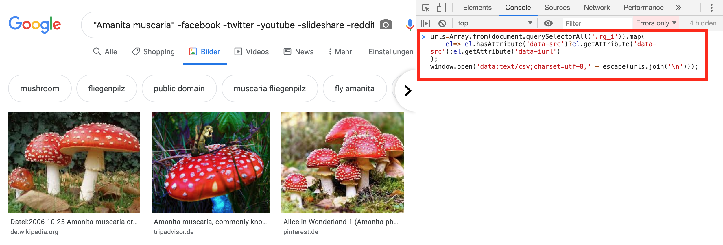
After running the code a file called Download.csv should get downloaded. This file contains the URLs of the images of the mushroom class you were searching for on Google. Let's rename the file to the corresponding class name. For instance, if I searched for images of the amanita muscaria, I will rename the file from Download.csv to amanita_muscaria.csv. You should end up with eight of these CSV files. One for each class. Finally, upload them to Google Drive. I chose to put them in a directory called urls, that I created in my base_dir directory (see above).
Now on Google Colab, we need to download the images using their URLs, that are stored in the eight CSV files. To do this we need to run the following steps for each mushroom class:
- Create a directory that is named according to the class.
- Take the corresponding CSV file with the image URLs and download each image by those URLs.
- Save the downloaded images into the created directory.
We should end up with eight directories. One for each mushroom class containing the corresponding images.
How can we do this in code? Fastai actually already provides a function called download_images, that takes a CSV file with image URLs and downloads the images by these URLs to a specified location. However, only images that can be opened are downloaded. To be able to execute download_images for each of the eight CSV files I wrote an own little wrapper function. This wrapper function takes a dictionary, which stores the class names as keys and the paths to the CSV files as values, and then loops over this dictionary to call download_images for each entry of the dictionary (i.e. each class).
def download_dataset(category_urls: Dict[str, Path], out_dir: Path, max_pics: int) -> None:
    categories = category_urls.keys()
    for c in categories:
        print('downloading images of class {}'.format(c))
        dest = out_dir/c
        url_file_path = category_urls[c]
        download_images(url_file_path, dest, max_pics=max_pics)
The dictionary with the class names as keys and the CSV file paths as values looks like the following.
category_urls = {
    'agaricus_campestris': base_dir + 'urls/agaricus_campestris.csv',
    'amanita_muscaria': base_dir + 'urls/amanita_muscaria.csv',
    'amanita_phalloides': base_dir + 'urls/amanita_phalloides.csv',
    'amanita_virosa': base_dir + 'urls/amanita_virosa.csv',
    'boletus_edulis': base_dir + 'urls/boletus_edulis.csv',
    'boletus_satanas': base_dir + 'urls/boletus_satanas.csv',
    'cantharellus_cibarius': base_dir + 'urls/cantharellus_cibarius.csv',
    'morchella_esculenta': base_dir + 'urls/morchella_esculenta.csv',
}

category_urls
Let's also store a list of the classes. To create such a list we simply need to take all the keys from our dictionary.
classes = list(category_urls.keys()); classes
Now let's specify where the directories for each class with the corresponding images should be stored. I decided to store them in a directory called data that I also created in the base_dir directory.
out_dir = Path(base_dir + 'data'); out_dir
Finally, we can call our wrapper function to download the images of the eight mushroom classes. Since I want to get as many images as possible, I specified to download maximally 700 images. We actually can't have more than 700 image URLs in each CSV file, since Google Images only gives us 700 at maximum.
download_dataset(category_urls, out_dir, 700)
Okay, let's check if the directories were created.
out_dir.ls()
This looks good. Now, let's go through all directories and check if some of the images are corrupted (e.g. since they couldn't be downloaded properly) or if they are okay and can be opened. If they are corrupted, we will remove them. Again, we don't need to code this all by ourselves. Fastai offers a function verify_images that checks all images of the directory and removes corrupted images. I just wrote a simply wrapper function again, that runs verify_images for all of our eight directories.
def remove_unaccessible_images(categories: List[str], ds_dir: Path) -> None:
    for c in categories:
        print('removing unaccessible images of class {}'.format(c))
        verify_images(ds_dir/c, delete=True, max_size=500)
        print()
Now, let's call the wrapper function.
remove_unaccessible_images(classes, out_dir)
According to the output there were no corrupted images found. If there have been any, we would have seen the file paths of them in the output. Next, let's load our dataset into an ImageDataBunch object. Since our dataset is structured among separate directories for the eight classes, we can use the from_folder method here. We split the dataset into 80% training and 20% validation set. Furthermore, we apply standard data augmentation and a normalization using ImageNet statistics to the data. This is similar to what I did when I trained a model to classify images of distracted drivers. For more information regarding how to load the data as an ImageDataBunch see my earlier blog post.
data = ImageDataBunch.from_folder(
    out_dir, train=".", valid_pct=0.2, ds_tfms=get_transforms(), size=224, num_workers=4
).normalize(imagenet_stats)
Let's check how many classes were loaded and how big our training and validation set is.
print('num classes:   {}'.format(data.c))
print('train_ds size: {}'.format(len(data.train_ds)))
print('valid_ds size: {}'.format(len(data.valid_ds)))
Good! All eight classes were loaded. Let's also display their class names.
data.classes
Finally, let's also look at a few images of our dataset.
data.show_batch(rows=3, figsize=(7,8))

Now, we are ready to train an initial model.
To train a mushroom classification model using our created dataset I am going to follow the same approach that I also used to train the model to classify images of distracted drivers. Thus, I will only briefly describe the training process here. Again, for more details check out my earlier blog post.
First, let's create a cnn_learner object with a ResNet50 network model architecture.
learn = cnn_learner(data, models.resnet50, metrics=accuracy)
We are going to use the 1-cycle-policy to train our model. Therefor, we need a maximum value for the learning rate hyper-parameter. To find a good value for the learning rate we can use the learning rate finder lr_find.
learn.lr_find()
learn.recorder.plot()

The minimum of the graph is at 1e-01. We should choose a number 10 times smaller than this minimum to set the learning rate. However, through some experiments I found out that 1e-03 works even a bit better here. Using this learning rate value let's train the last layer of the network for 6 epochs now.
learn.fit_one_cycle(6, max_lr=1e-03)
We reached an accuracy of 83.74%. This is not too bad. Let's save our model.
learn.save('stage-1')
Then, let's unfreeze all the layers and train the whole network for 12 more epochs. For the deeper layers I keep using the learning rate value that we found by using the learning rate finder. For the earlier layers we should use a value ten times smaller than that for the learning rate.
learn.unfreeze()
learn.fit_one_cycle(12, max_lr=slice(1e-4,1e-3))
We could improve our model up to 87.04% accuracy. Let's save our model.
learn.save('stage-2')
Next, let's see which mistakes our model makes. We can use the ClassificationInterpretation class for this. It will give us the samples of the validation set with the highest losses.
interp = ClassificationInterpretation.from_learner(learn)
losses, idxs = interp.top_losses()
Let's plot the images with the highest losses.
interp.plot_top_losses(9, figsize=(15,11))

Okay, as we can see we have some problems with our dataset. We have some weird images like e.g. the first image in the second row, which shouldn't be in our dataset. Furthermore, we also have images with incorrect labels like e.g. the first image in the first row. It's clearly an Amanita Muscaria and our model also recognized that correctly. However, that image is labeled incorrectly as Amanita Virosa. Well, that we don't get a clean, ready-to-use image dataset using Google Images is actually not surprising. So, we need to clean the data! However, before we do that let's also plot the confusion matrix for completeness.
interp.plot_confusion_matrix(figsize=(12,12), dpi=60)

Additionally, let's also plot the classes our model gets most confused about.
interp.most_confused(min_val=2)
Now, let's clean our dataset.
To clean the dataset we can use a widget provided by fastai that is called ImageCleaner. This widget will make the cleaning process a lot easier.
For cleaning the data we don't need to have it split into a training and validation set. Moreover, we also don't want to normalize the data, since we want to look at the original unchanged images. We want to load and then look at them to be able to decide whether we want to remove an image from the dataset or if we need to change an image's label. So, let's create a new ImageDataBunch object without the splitting and normalization.
data_bunch = (
    ImageList.from_folder(out_dir)
        .split_none()
        .label_from_folder()
        .transform(get_transforms(), size=224)
        .databunch()
)
Now, we are ready to clean the data. As I mentioned before our trained model will help us cleaning the dataset. So, let's create a new cnn_learner and load our model. However, this time we are not going to use it for model training.
learn_cln = cnn_learner(data_bunch, models.resnet50, metrics=accuracy)
learn_cln.load('stage-2');
So, why is our model useful for cleaning the data? Well, we can use our model to find the images for which our model gives high losses. A high loss means either a) our model is not very good or b) something is wrong with the image (e.g. weird image, wrong image label). Thus, let's check the images with a high loss. To obtain these images we can use the from_toplosses method of the DatasetFormatter class.
ds, idxs = DatasetFormatter().from_toplosses(learn_cln)
Now, we can use the ImageCleaner widget on the images with high losses. After executing the following command a graphical menu like the one below will appear. It shows four images of our dataset that resulted in a high loss. Below each image is a button Delete. By clicking on that button we can remove that image from the dataset. Moreover, there is also a drop down list containing the mushroom labels below each image, which makes it possible to change the label of that image. When we are done with these four images, we can click Next Batch to receive the next four images, which we can check as well. We can repeat this process until there are no more images left. In this case the message No images to show :) will appear.
ImageCleaner(ds, idxs, out_dir)

Besides images that don't show mushrooms we also don't want to have duplicate images in our dataset. The DatasetFormatter also has a method from_similar to give us similar images of our dataset indicating that these images could be duplicates. The similarity scores are computed from the layer activations of our network.
ds, idxs = DatasetFormatter().from_similars(learn_cln)
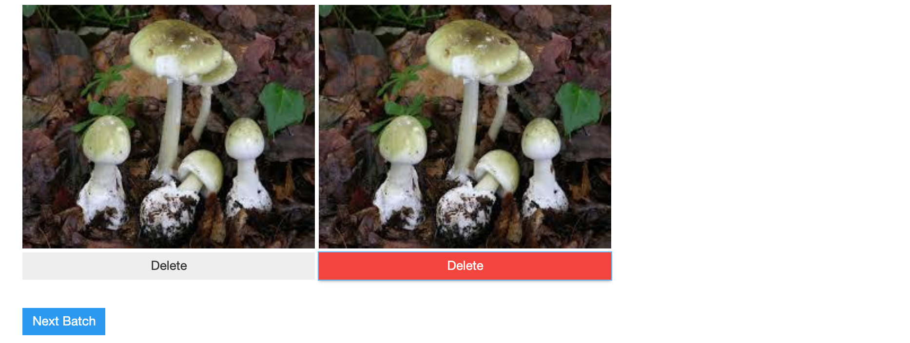
Now we can use the ImageCleaner widget again. This time it will show a graphical menu like the one below that always shows us a pair of images. Again, by clicking the Delete button we can remove an image from the dataset. After we decided whether we want to delete one of the two images (i.e. in case of duplicate images) or not we can click on Next Batch and the widget will show us the next pair of images. This process repeats until there are no more images. In this case the message No images to show :) will appear.
ImageCleaner(ds, idxs, out_dir, duplicates=True)
However, the images we decided to remove from the dataset are actually not deleted from our hard drive. Instead, the widget creates a CSV file called cleaned.csv, which only contains the images we didn't want to have removed from the dataset as well as their corrected labels.
By the way, the cleaning process can actually take quite some time. If you decide to take a break in between, you can simply use the current cleaned.csv file to create a new ImageDataBunch object using the from_csv method when you want to continue cleaning (instead of the from_folder method that we used before).
data_bunch = (
    ImageList.from_csv(out_dir, 'cleaned.csv')
        .split_none()
        .label_from_folder()
        .transform(get_transforms(), size=224)
        .databunch()
)
When we finished the cleaning, we can train a new model with out cleaned dataset.
Let's use the cleaned.csv CSV file to load the dataset. So, let's create an ImageDataBunch object from that CSV file using the method from_csv. We split the dataset into 80% training and 20% validation set again. Moreover, we also apply basic data augmentation as well as normalization using the ImageNet statistics to the images of our dataset as before.
data = ImageDataBunch.from_csv(
    ds_dir, folder=".", valid_pct=0.2, csv_labels='cleaned.csv',
    ds_tfms=get_transforms(), size=224, num_workers=4
).normalize(imagenet_stats)
Now, let's check how big our training and validation set is.
print('num classes:   {}'.format(data.c))
print('train_ds size: {}'.format(len(data.train_ds)))
print('valid_ds size: {}'.format(len(data.valid_ds)))
It got a lot smaller! Well, I needed to remove a lot of images from the dataset. But let's check if we still have images of all eight classes.
data.classes
Okay, we do have images of all eight classes. Let's also look at a few images of the dataset.
data.show_batch(rows=3, figsize=(7,8))

We can't see any strange images, which is a good sign. However, these are only nine images of our dataset. Let's train the model to see whether we can train a better model using our cleaned data this time. First, let's create a cnn_learner with a ResNet50 network architecture again.
learn = cnn_learner(data, models.resnet50, metrics=accuracy)
Then, let's find the learning rate for the 1-cycle-policy.
learn.lr_find()
learn.recorder.plot()

The value 1e-03 seems still to be a good value for the learning rate here. So, let's train the last network layer with that learning rate value for six epochs.
learn.fit_one_cycle(6, max_lr=1e-03)
Oh! We could improve a lot compared to our initial model. Let's save the current model.
learn.save('stage-3')
Now, we should unfreeze our model and train for 12 more epochs.
learn.unfreeze()
learn.fit_one_cycle(12, max_lr=slice(1e-4,1e-3))
Okay. We have been able to improve even a bit further to an accuracy of about 98.14%. Let's safe the model!
learn.save('stage-4')
Although our new model was able to reach over 98% accuracy, we should take a look into where our model makes mistakes.
interp = ClassificationInterpretation.from_learner(learn)
losses, idxs = interp.top_losses()
interp.plot_top_losses(9, figsize=(15,11))

As we can see the first two images of the first row still have a wrong label. I must have missed them when I cleaned the dataset. The other mistakes are not very surprising, since our model mixes up classes of mushrooms that a very similar (e.g. Agaricus Campestris and Boletus Edulis). Let's also look at the confusion matrix.
interp.plot_confusion_matrix(figsize=(12,12), dpi=60)

interp.most_confused(min_val=2)
This looks quite good actually. We trained a model that is able to classify images of mushrooms with an accuracy of over 98% on the validation set using an own image dataset for model training.
cnn_learner). This pretrained model was originally trained on 1000 ImageNet classes including a general mushroom class. Although it was not trained to distinguish different mushroom types, it probably at least knew something about mushrooms already.
However, although our model reaches an accuracy of over 98%, our model needs to tested on way more data before it can be used in practice. Furthermore, it would be also important that our classifier let's us know if it doesn't know a mushroom we show it. I only included eight types of mushrooms for our model, but there exist way more of course. Currently, our classifier would simply predict any of the eight classes when it sees an unknown mushroom type. So, be cautious. Mixing up mushroom can be dangerous! However, since the focus of this blog post is on creating an own training dataset and not on how to create a ready-to-use mushroom classifier, we are done for now.